4.7 Other kinds of limit

Limit at infinity

The ‘limit at infinity’ of a function tells us how $f(x)$ behaves for large values of $x$ .

Definition 4.64.

Let $I\subseteq\mathbb{R}$ be an interval which is not bounded above and $f\colon I\to\mathbb{R}$ . We say $f(x)$ converges to $\ell\in\mathbb{R}$ as $x\to\infty$ if for all $\varepsilon>0$ , there exists some $R>0$ (which in general depends on $\varepsilon$ ) such that

\text{if $x\in I$ satisfies $x>R$, then}\quad|f(x)-\ell|<\varepsilon.

In this case, we write $\displaystyle\lim_{x\to\infty}f(x)=\ell$ or $f(x)\to\ell$ as $x\to\infty$ .

Definition 4.64 is clearly very similar to the $\varepsilon$ - $N$ definition of a limit of a sequence. Indeed, the following example shows how proofs based on this “ $\varepsilon$ - $R$ ” definition look very similar to the “ $\varepsilon$ - $N$ ” proofs from Chapter 2.

Example 4.65.

$\displaystyle\lim_{x\to\infty}\tfrac{x}{x^{2}+1}=0$ .

Proof.

Let $\varepsilon>0$ be given and choose $R:=\frac{1}{\varepsilon}>0$ . If $x>R$ , then

0\leq\frac{x}{x^{2}+1}\leq\frac{x}{x^{2}}=\frac{1}{x}<\frac{1}{R}=\varepsilon.

Hence, by the $\varepsilon$ - $R$ definition of a limit, $\displaystyle\lim_{x\to\infty}\tfrac{x}{x^{2}+1}=0$ . ∎

Exercise 4.66.

By arguing from the definition, show that $\displaystyle\lim_{x\to\infty}\tfrac{3x^{2}+5x+2}{2x^{2}+x+4}=\tfrac{3}{2}$ .

One way to interpret the result of Example 4.65 is that the function $x^{2}+1$ grows much faster than the function $x$ , which means that the ratio $\frac{x}{x^{2}+1}$ gets very small for large values of $x$ .

A key property of the exponential is that it grows very quickly as $x$ gets large: faster than any polynomial! On the other hand, the natural logarithm function grows very slowly: slower than any power! From this, we expect, for instance,

(4.13) (4.13)

\lim_{x\to\infty}\frac{x^{2}}{\exp(x)}=0\qquad\text{and}\qquad\lim_{x\to\infty% }\frac{(\log x)^{100}}{x}=0.

In order to prove statements such as those in (4.13), we introduce the following lemma which describes the behaviour of $\exp(x)$ and $\log(x)$ for large values of $x$ .

Lemma 4.67 (Asymptotics for

\exp

and

\log

Let $n\in\mathbb{N}$ and $M>0$ . Then there exists $R$ , $S\geq 1$ , depending on $n$ and $M$ , such that

1

$\exp(x)>Mx^{n}$ for all $x>R$ ;
2

$\log(y)<M^{-1}y^{1/n}$ for all $y>S$ .

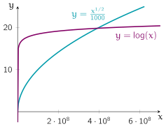
Here the word ‘asymptotics’ is used to mean ‘behaviour for large values of $x$ or $y$ ’. To illustrate Lemma 4.67 (i), take $n=2$ and $M=1000$ . Then we see that there exists some $R\geq 1$ such that $\exp(x)>1000x^{2}$ for all $x>R$ . In other words, eventually (that is, for all values of $x>R$ ), the function $\exp$ is much larger (by a factor of $1000$ ) than the function $x\mapsto x^{2}$ . Similarly, Lemma 4.67 (ii) tells us that eventually the function $\log$ is much smaller than the function $y\mapsto y^{1/2}/1000$ . These relationships are illustrated in Figure 4.18.

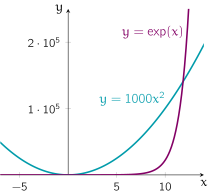
(a) For large enough

x

\exp(x)>1000x^{2}

(b) For large enough

x

\log(x)<\frac{x^{1/2}}{1000}

Figure 4.18: Examples illustrating the asymptotics of

\exp

and

\log

Proof (of Lemma 4.67).

Fix $n\in\mathbb{N}$ and $M>0$ .

1. By the definition (4.2) of the exponential function,

\exp(x):=\sum_{k=0}^{\infty}\frac{x^{k}}{k!}\geq\frac{x^{n+1}}{(n+1)!}=\frac{x% }{(n+1)!}\cdot x^{n}\qquad\text{for all $x\geq 0$,}

where we have used the fact that all the summands are non-negative. If we set $R:=M(n+1)!$ , then it immediately follows that $\exp(x)>Mx^{n}$ for all $x>R$ , as required.

2. By applying part 1 with $M$ replaced with $M^{n}$ , there exists some $R\geq 1$ such that

\exp(x)>M^{n}x^{n}\qquad\text{for all $x>R$.}

Substituting $x=\log y$ yields

y=\exp(\log y)>M^{n}(\log y)^{n}\qquad\text{for all $y\in\mathbb{R}$ such that% $\log y>R$.}

Since $\log$ is an increasing function, if we set $S:=\exp(R)$ and choose $y>S$ , then $y>M^{n}(\log y)^{n}$ for all $y>S$ , which rearranges to give the desired inequality. ∎

We can now use Lemma 4.67 to prove limit identities involving $\exp$ and $\log$ .

Example 4.68.

$\displaystyle\lim_{x\to\infty}\tfrac{x^{2}}{\exp(x)}=0$ .

Proof.

Let $\varepsilon>0$ be given. By Lemma 4.67, there exists some $R>0$ such that $\exp(x)>\varepsilon^{-1}x^{2}$ for all $x>R$ . If $x>R$ , then

0\leq\frac{x^{2}}{\exp(x)}<\frac{x^{2}}{\varepsilon^{-1}x^{2}}=\varepsilon.

Hence, by the $\varepsilon$ - $R$ definition of a limit, $\displaystyle\lim_{x\to\infty}\tfrac{x^{2}}{\exp(x)}=0$ . ∎

Exercise 4.69.

Show that

(i)

$\displaystyle\lim_{x\to\infty}\frac{\exp(x)+10x^{3}+4x^{2}}{\exp(x)}=1$ ;
(ii)

$\displaystyle\lim_{x\to\infty}\frac{(\log x)^{100}}{x}=0$ .

One-sided limits

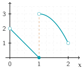
Consider the function $j$ illustrated in Figure 4.19. We can see this has a discontinuity at $x=1$ . However, if we imagine approaching $1$ from the left-hand side by considering $f(x)$ for larger and larger values of $x$ satisfying $x<1$ , then the function does appear to converge to a limit, corresponding to the solid blue dot at $(1,0)$ .

Figure 4.19: The function

j\colon(0,2)\to\mathbb{R}

from Example 4.73 has a jump discontinuity at

x=1

To make this idea precise, we introduce the notion of a one-sided limit.

Definition 4.70.

Let $I\subseteq\mathbb{R}$ be an interval and $a\in I$ . Let $f\colon E\to\mathbb{R}$ where either $E=I$ or $E=I\setminus\{a\}$ .

1

Suppose $a$ is not the left endpoint of $I$ . We say $f(x)$ converges to $\ell\in\mathbb{R}$ from the left if for all $\varepsilon>0$ , there exists some $\delta>0$ such that

$\text{if $x\in I$ satisfies $a-\delta<x<a$, then}\quad|f(x)-\ell|<\varepsilon.$

In this case, we write $\displaystyle\lim_{x\to a_{-}}f(x)=\ell$ or $f(x)\to\ell$ as $x\to a_{-}$ .
2

Suppose $a$ is not the right endpoint of $I$ . We say $f(x)$ converges to $\ell\in\mathbb{R}$ from the right if for all $\varepsilon>0$ , there exists some $\delta>0$ such that

$\text{if $x\in I$ satisfies $a<x<a+\delta$, then}\quad|f(x)-\ell|<\varepsilon.$

In this case, we write $\displaystyle\lim_{x\to a_{+}}f(x)=\ell$ or $f(x)\to\ell$ as $x\to a_{+}$ .

Example 4.71.

Consider the function $j\colon(0,2)\to\mathbb{R}$ given by

j(x):=\begin{cases}2(1-x)&\text{for $0<x\leq 1$,}\\ 3-2(1-x^{2})&\text{for $1<x<2$;}\end{cases}

we sketch the graph of this function in Figure 4.19.

Left-hand limit. Let $\varepsilon>0$ be given and choose $\delta:=\min\{1,\varepsilon/2\}$ . If $1-\delta<x<1$ , then

|j(x)|=2(1-x)<2\delta\leq\varepsilon.

Hence $\displaystyle\lim_{x\to 1_{-}}j(x)=0$ by the $\varepsilon$ - $\delta$ definition of a one-sided limit.

Right-hand limit. Let $\varepsilon>0$ be given and choose $\delta:=\min\{1,\varepsilon/6\}$ . If $1<x<1+\delta$ , then

|j(x)-3|=2(x^{2}-1)=2(1+x)(x-1)<2\cdot 3\cdot\delta\leq\varepsilon.

Here we used the fact that $x<2$ , which implies that $1+x<3$ , and the fact that $x<1+\delta$ , which implies that $x-1<\delta$ .

Hence $\displaystyle\lim_{x\to 1_{+}}j(x)=3$ by the $\varepsilon$ - $\delta$ definition of a one-sided limit.

One-sided limits are related to regular limits of functions via the result of the following exercise.

Exercise 4.72.

Let $I\subseteq\mathbb{R}$ be an interval and $a\in I$ . Assume $a$ is not an endpoint of $I$ . Let $f\colon E\to\mathbb{R}$ where either $E=I$ or $E=I\setminus\{a\}$ . Show that the following are equivalent:

1.

The limit $\displaystyle\lim_{x\to a}f(x)$ exists and satisfies $\displaystyle\lim_{x\to a}f(x)=\ell$ ;
2.

The left limit $\displaystyle\lim_{x\to a_{-}}f(x)$ and the right limit $\displaystyle\lim_{x\to a_{+}}f(x)$ both exist and satisfy

$\lim_{x\to a_{-}}f(x)=\lim_{x\to a_{+}}f(x)=\ell.$

This characterisation is often convenient for showing limits do not exist, by demonstrating a discrepancy between the left and right limits.

Example 4.73.

Consider the function $j\colon(0,2)\to\mathbb{R}$ as in Example 4.71. As we saw above, the left and right-hand limits of $j$ at $0$ both exist but

\lim_{x\to 1_{-}}j(x)=\lim_{x\to 1_{-}}2(1-x)=0\qquad\text{and}\qquad\lim_{x% \to 1_{+}}j(x)=\lim_{x\to 1_{+}}3-2(1-x^{2})=3.

Since the one-sided limits do not agree, by applying the result of Exercise 4.72, the limit $\displaystyle\lim_{x\to 1}j(x)$ does not exist.

Exercise 4.74.

Let $f\colon(0,\infty)\to\mathbb{R}$ be given by

f(x):=\begin{cases}\sin\big{(}\pi/(2x)\big{)}&\text{if $0<x<1$;}\\ -1485&\text{if $x=1$;}\\ x^{2}&\text{if $x>1$.}\end{cases}

Determine whether each of the limits $\displaystyle\lim_{x\to 1_{+}}f(x)$ , $\displaystyle\lim_{x\to 1_{-}}f(x)$ and $\displaystyle\lim_{x\to 1}f(x)$ exist and (if they do exist) compute their values. Is $f$ continuous at $1$ ?

Hint: $\displaystyle\lim_{x\to 1_{-}}f(x)$ is tricky (but will become easier once we’ve studied the limit laws). As the first step, try to use the fact $\sin\colon\mathbb{R}\to\mathbb{R}$ is continuous.

Tending to infinity

The function $x\mapsto 1/x^{2}$ blows up as $x$ approaches $0$ : see Figure 4.20. This is often called a vertical asymptote and is described precisely using another kind of limit.

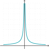
Figure 4.20: The function

f\colon\mathbb{R}\setminus\{0\}\to\mathbb{R}

given by

f(x):=1/x^{2}

Definition 4.75.

Let $I\subseteq\mathbb{R}$ be an interval, $a\in I$ and $f\colon I\setminus\{a\}\to\mathbb{R}$ . We say $f$ tends to $\infty$ as $x$ tends to $a$ if for all $M>0$ there exists some $\delta>0$ such that

\text{if $x\in I$ satisfies $0<|x-a|<\delta$, then}\quad f(x)>M.

In this case, we write $\displaystyle\lim_{x\to a}f(x)=\infty$ or $f(x)\to\infty$ as $x\to a$ .

Warning 4.76.

As always, here ‘ $\infty$ ’ is merely part of the notation. It is just a symbol and does not represent a number or any other mathematical object.

Exercise 4.77.

Give an informal explanation of what it means for $\lim_{x\to a}f(x)=\infty$ and match it to the precise definition by filling in the following table.

$M$ - $\delta$ definition (4.4)	Informal idea
For all $M\in\mathbb{R}$
there exists some $\delta>0$
such that if $x\in I$ satisfies $0<\|x-a\|<\delta$ ,
then $f(x)>M$ .

Example 4.78.

$\displaystyle\lim_{x\to 1}\frac{3}{x^{2}-1}=\infty$

Proof.

For $x\in\mathbb{R}\setminus\{1,-1\}$ , we may write

\frac{3}{x^{2}-1}=\frac{3}{x+1}\cdot\frac{1}{x-1}.

Suppose $0<|x-1|<1$ . From this we can deduce that $0<x<2$ , so $1<x+1<3$ and therefore $\frac{3}{x+1}>1$ . Thus in this case,

\Big{|}\frac{3}{x^{2}-1}\Big{|}=\frac{3}{x+1}\cdot\frac{1}{|x-1|}>\frac{1}{|x-% 1|}.

Let $M\in\mathbb{R}$ be given and choose $\delta:=\min\{1/M,1\}$ . If $0<|x-1|<\delta$ , then $0<|x-1|<1$ and so it follows by our earlier observations that

\Big{|}\frac{3}{x^{2}-1}\Big{|}>\frac{1}{|x-1|}\geq\frac{1}{|x-1|}>\frac{1}{% \delta}\geq M.

Since $M>0$ was chosen arbitrarily, by definition $\lim_{x\to 1}\frac{3}{x^{2}-1}=\infty$ . ∎

Exercise 4.79.

Verify the following limit identities.

(i)

$\displaystyle\lim_{x\to 3}\frac{5x}{(x^{3}-27)^{2}}=\infty$ ;
(ii)

$\displaystyle\lim_{x\to 0}\frac{|\sin x|}{x^{2}}=\infty$ .

There are many other kinds of limit, some of which can be obtained by mixing and matching existing definitions. Rather than write out a comprehensive list, we leave you to think about how you would go about formalising the definitions.

Exercise 4.80.

Let $I\subseteq\mathbb{R}$ be an interval and $a\in I$ . Assume $a$ is not an endpoint of $I$ and let $f\colon I\setminus\{a\}\to\mathbb{R}$ . Write down a sensible definition of what it means for the following to hold.

(i)

$\displaystyle\lim_{x\to a}f(x)=-\infty$ ;
(ii)

$\displaystyle\lim_{x\to a_{+}}f(x)=\infty$ ;
(iii)

$\displaystyle\lim_{x\to a_{-}}f(x)=-\infty$ .

Exercise 4.81.

Write down a sensible definition of what it means for $f\colon\mathbb{R}\to\mathbb{R}$ to satisfy the following.

(i)

$\displaystyle\lim_{x\to\infty}f(x)=\infty$ ;
(ii)

$\displaystyle\lim_{x\to-\infty}f(x)=\infty$ .

Exercise 4.82.

Arguing from the definitions you came up with in Exercise 4.80 and Exercise 4.81, verify the following limit identities.

(i)

$\displaystyle\lim_{x\to 0_{+}}\frac{1}{x}=\infty$ ;
(ii)

$\displaystyle\lim_{x\to 0_{-}}\frac{1}{x}=-\infty$ ;
(iii)

$\displaystyle\lim_{x\to\infty}\exp(x)=\infty$ .

Limit laws

There are versions of the limit laws for each kind of limit introduced above. We shall not write out formal theorem statements of all of these laws (since to do so would be rather repetitive), but content ourselves with an illustrative example.

Example 4.83.

$\displaystyle\lim_{x\to 0_{+}}x\log x=0$ .

Proof.

Here we use the composition law to change variables. In particular, writing $x=1/u$ , we obtain

x\log x=\frac{\log(1/u)}{u}=-\frac{\log u}{u}.

Here we have used the familiar property of the logarithm that $\log(1/u)=-\log u$ . Strictly speaking, we have not yet shown that our definition of $\log$ satisfies this property, but we shall prove this is the case in the next chapter.

Given $\varepsilon>0$ , by Lemma 4.67 we know there exists some $S\geq 1$ such that $\log u<\varepsilon u$ for all $u>S$ . Thus, $0\leq\log u/u<\varepsilon$ for all $u>S$ and therefore, by the definition of a limit, $\displaystyle\lim_{u\to\infty}\tfrac{\log u}{u}=0$ .

Finally, since $\displaystyle\lim_{u\to\infty}\tfrac{\log u}{u}=0$ and $x=1/u\to 0$ as $u\to\infty$ , it follows from the composition law that $\displaystyle\lim_{x\to 0_{+}}x\log x=0$ , as required. ∎

Exercise 4.84.

Show that $\displaystyle\lim_{x\to\infty}x^{2}\sin(1/x^{2})=1$ .